
April 2024 / RETIREMENT INSIGHTS
How Do You Evaluate a Glide Path?
Glide path evaluation is not an easy task.
Key Insights
- In evaluating target date glide paths, T. Rowe Price looks at economic utility—their potential to satisfy investors’ retirement income and wealth preferences.
- A numerical utility score means relatively little to most investors. So our model generates metrics that measure possible retirement outcomes more directly.
- We believe the metrics in our evaluation process make it easier for plan sponsors and investors to assess whether a glide path reflects their own preferences.
Over the course of two decades of research, T. Rowe Price has developed a proprietary framework for glide path design that is centered on a structural model incorporating the inputs, parameters, and mathematical techniques that we believe are necessary to represent accurately the challenges faced by retirement investors.
In a previous T. Rowe Price Insights paper, we highlighted certain aspects of our model to demonstrate how we evaluate the range of possible outcomes associated with a particular glide path.1 As we progress through our Making the Benefit Connection series, this information will be essential to understanding how the presence of defined benefit (DB) plans potentially affect the appropriate level and shape of the glide paths for target date offerings in companion defined contribution (DC) plans.
The primary metric that T. Rowe Price uses to evaluate a glide path design is economic utility, which measures the degree of satisfaction a person experiences from possessing or consuming an economic good. In the case of glide path evaluation, the economic goods in question are income for spending and accumulated wealth. Income and wealth both provide levels of satisfaction that can be measured in terms of investor utility. And, in both cases, there is a governing principle that economic theory typically treats as universal: the law of diminishing marginal utility.
To illustrate this principle, consider a simple example involving a favorite meal. Even though the entire meal is satisfying, the last bite will not be as satisfying as the first bite. While we address this issue mathematically—which provides a rigorous way to combine our utility model’s many features—our approach also fits naturally with the way we prefer to express the problem: How can we potentially make an investor as satisfied as possible given their preferences? As John Dewey, the prominent American philosopher, once said: “A problem well‑put is half‑solved.” 2
Utility is based on a set of individualized preferences. However, expressed simply as a number, the concept has relatively little meaning for the typical investor, in our view. To convey why certain glide paths potentially are appropriate for specified preferences, we have compiled a set of complementary metrics to express possible retirement outcomes. Our metrics measure risk and reward in ways that we believe investors actually care about, rather than simply in terms of portfolio return and volatility.
In our view, the metrics generated using our model make it easier for plan sponsors to assess whether, on balance, a particular glide path reflects their preferences. However, we recognize that this might not be obvious on first impression. So, instead of focusing on just one glide path, our model analyzes a range of glide paths that takes into consideration slight adjustments to investor preferences and the potential trade‑offs associated with those choices. We refer to this spectrum of glide paths as a “suitability range.”
To help explain the benefits of utility theory, we first argue for the need for a more capable approach than those typically in use today. We then provide a high‑level explanation of our utility model. Finally, we explain some of the model’s key inputs, including preference values and plan demographics, and discuss our results metrics and our suitability range. We believe this discussion will help lay a solid foundation for understanding the effects of DB plans on companion DC plans.
Two important effects
Earned pension benefits often are similar in nature to Social Security benefits. Both payment streams represent deferred labor income that has a measurable present value. An investor receiving defined benefits has a higher guaranteed fixed income than another investor with the same salary and financial capital but no DB plan. Assuming the two individuals are using the same DC glide path, the investor receiving defined benefits, in effect, has a higher overall fixed income allocation.
Other things being equal, this dynamic suggests that to be properly diversified across all their assets, investors receiving defined pension benefits should shift more of their financial capital to equity‑like assets (i.e., they should have higher equity‑like exposures in their DC glide paths) to adjust for the effect of their defined benefits on their overall allocations. We call this the “substitution effect.”
The substitution effect may seem relatively straightforward, but does it actually make sense? Suppose, for example, that two investors have identical salaries, savings rates, employer matching contribution rates, and account balance histories. However, one also receives significant payments from a DB plan.
- Clearly, the individual with the DB plan should be able to expect a more securely funded retirement than the person without a DB plan.
- Greater income security should mean that the DB plan beneficiary has less need for the potential long‑term growth advantages conveyed by higher equity exposure.
- Being risk averse, the DB beneficiary ordinarily could be expected to lower equity exposure rather than raise it.
For our hypothetical defined benefit recipient, the outcome of the utility function is the opposite of the one predicted by the substitution effect—equity exposure in the preferred glide path should be lower rather than higher. We call this offsetting preference the “wealth effect.”
These arguments are cogent because our research confirms that the substitution and wealth effects are both real. Their relative strengths are tied to individual preferences and circumstances that need to be assessed and considered together. To incorporate both effects in a parsimonious glide path design model, we must develop a rich and nuanced approach to glide path evaluation. We explore this concept further in the fourth paper in this series.
Seeking to maximize investor utility
The personality traits that influence economic satisfaction are tied to certain goals and preferences that help define that person. Everyone has a unique blend of these preferences. In our view, the utility function is a rigorous way to describe the interactions of these characteristics and to measure the level of satisfaction a given set of outcomes can provide an individual.
We measure these preferences with explicit parameters. Furthermore, our model ascribes utility to two distinct sources. On the one hand, people enjoy the goods they consume that are paid for out of their retirement savings. Measuring utility as a function of consumption is a common approach. However, we believe that people also derive value from the security, flexibility, and autonomy derived from maintaining or growing their wealth.
Uniquely, our model factors both sources of satisfaction into its utility score. However, reflecting the contravening dynamics of seeking to both maintain and consume wealth, efforts to increase the utility score by improving investors’ outcomes along one of these two dimensions inherently come at the expense of the other. Individual preferences are used to establish a tipping point that seeks to balance the two sources of utility in a unique way for each person or group of people.
Behavioral preferences are just one of three classes of variables simulated in our framework (Figure 1). Capital market assumptions and demographic factors also play key roles.
T. Rowe Price’s glide path designs are based on three input types
(Fig. 1) Input classes

Source: T. Rowe Price.
T. Rowe Price has built a proprietary cascading model for generating capital market returns based on economic factors and calibrated to certain assumptions. While this is an essential design component, unless a plan sponsor has a significantly different outlook for asset class returns compared with our inputs, different capital market assumptions are relatively less important for differentiating glide paths and their suitability.
Far more influential are demographic characteristics and behaviors. We model investor cash flows including income, savings, Social Security benefits, and behaviorally representative spending patterns. These draw on our capital markets model but also incorporate mortality rates and employer matches. Changes in these flows can meaningfully impact the indicated shape of a glide path.
To tie all of these variables together, we use Monte Carlo simulation to generate thousands of hypothetical scenarios for quantities such as macroeconomic variables, asset class returns, salary trajectories, portfolio balance growth, spending policies in retirement, and sampled preference values. The suggested glide path is the one that provides the highest utility for a population described by its behavioral preferences and demographics under our definition of utility. We then use the hypothetical outcomes produced by the suggested glide path as inputs to the set of metrics we cited at the beginning of this paper and that we will discuss in more detail later.
Our approach allows us to incorporate these three classes of inputs into objective criteria and apply a consistent investment evaluation process across a variety of retirement goals and expectations.
Preferences, demographics, and their impact
In this section, we will explain which preferences we include in our utility function and how they potentially interact with the presence of a DB plan to impact the level and shape of the appropriate glide path (Figure 2). We also will discuss a measure of retirement preparedness that similarly bears on the effect of a DB plan.
DB plans can affect glide path design at both individual and plan levels
(Fig. 2) Preferences that potentially influence glide path utility

Source: T. Rowe Price.
Consumption vs. wealth
The fundamental trade‑off between consumption and wealth manifests itself at two levels, which can be expressed as two individual preferences. The first of these preferences is a natural aversion to depleting wealth. Some individuals prefer to seek to maintain greater control of their wealth by consuming less, while others will accept partial depletion of their wealth over time in order to pay for greater consumption. Depletion aversion measures the first preference: the behavioral resistance to spending from one’s savings.
The second preference incorporated in our utility function involves the relative importance placed on limiting exposure to market fluctuations—especially near retirement—compared with the priority of seeking growth to pay for higher average consumption in retirement. Historically, the higher returns generated by equities helped finance greater consumption levels over time; however, the historically higher variability of equity returns may expose portfolio balances to greater risk in the short term. The investment goal of a glide path reflects the plan sponsor’s priorities in this regard.
Benefits from a DB plan can supplement consumption without depleting the individual’s DC plan balance. This potentially impacts the associated glide path through both the wealth and the substitution effects.
Planning horizon
Another preference for plan sponsors to consider is the planning horizon of their participants. The shorter the planning horizon, the more valuable is satisfaction in the near future relative to satisfaction in more distant time periods. The shorter the horizon, the less the need for equity in the glide path to provide the growth to fund distant future utility. A lifetime defined benefit provides a guaranteed income floor, which may lower participants’ patience for spending their hard‑earned savings and further reduce the suggested level of equity exposure in the glide path.
Risk aversion
We also explicitly represent risk aversion in our utility function. This establishes a trade‑off between the level of average consumption and the risk of below‑average consumption levels. Greater risk aversion tends to reduce the appropriate level of equity in the glide path. However, it is important to note that risk aversion is not the same as risk perception. Two different people can perceive the same amount of risk in one situation, but their responses will depend on how averse they are to taking risks. A given level of risk might be palatable for one investor while another might find it unacceptably high.
By allowing plan participants to rely less heavily on their portfolio balances for income, a DB plan potentially lowers the amount of risk that the investor perceives in their glide path. However, it does not change their innate risk preferences.
Retirement preparedness
Our demographic behavior model is focused on how reliant participants are on their DC plans to support their expected future income needs and on how well they are using their plans to prepare for retirement.
As a measure of an investor’s reliance on in‑plan assets to support nondiscretionary retirement spending, we often use the ratio of assets to salary. The evolution of this ratio through time tracks an investor’s progress toward the desired retirement outcomes by answering a simple question: “How many years of my current salary do I currently have saved?”
A relatively low asset‑to‑salary ratio (perhaps reflecting lower past contributions and/or depressed portfolio returns) means the investor is less well prepared for retirement, which in turn implies a higher‑equity glide path in our model. Other things being equal, the presence of a DB plan improves the asset‑to‑salary ratio because the present value of accrued future benefits effectively increases the investor’s total assets, implying that a lower‑equity glide path is more appropriate. The relative strengths of these effects when they are coincident is not straightforward.
Robust results
Our comments above focused on individual preferences. However, we also recognize that glide paths typically are designed for diverse populations of investors and that preferences will vary among those individuals. Even for a single investor, preferences can be difficult to measure precisely. Therefore, we represent each preference as a separately calibrated distribution of values rather than as a single average value. We believe this approach makes our results much more robust to changes in parameter values. Small changes should not cause big changes in the model’s outputs, which we believe makes our solutions broadly applicable for heterogeneous populations. We discussed this aspect of our process in more detail in a previous T. Rowe Price Insights paper.3
Meaningful metrics and the range of suitable glide paths
The metrics we present to a plan sponsor, taken as a whole, encapsulate the trade‑offs between participant preferences in order to convey the appropriateness of a given glide path. For consistency with our utility function, and for the same underlying reasons, our metrics measure quantities that are related to both consumption and wealth. For each metric, we provide an indication of potential reward and risk.
To be meaningful, the metrics we use need to be easy to understand and relevant to the perspective of an investor. As the array of preferences discussed above suggests, this goes beyond the total return and market volatility metrics typically considered in standard financial theory (Figure 3).
Investors care about metrics that are relevant to their retirement goals
(Fig. 3) Reward and risk metrics for consumption and wealth
|
Consumption |
Wealth |
Reward |
Consumption Replacement |
Wealth at Retirement |
Risk |
Expected Shortfall |
Maximum Drawdown |
Source: T. Rowe Price
Consumption
The primary goal of saving for retirement is to be able to replace some desired percentage of preretirement income for the rest of the investor’s life. The consumption replacement metric indicates what percentage of income an individual potentially can expect to replace by following a given glide path, taking into account all potential sources of retirement‑related income. These sources may include Social Security benefits, annuity payments, defined benefits, and withdrawals from savings.
The consumption replacement metric is derived from forecasted spending patterns that are weighted by mortality. These spending patterns are derived from our dynamic spending model, which adjusts projected retirement consumption based on the internal economic and demographic state of the simulation. 4 We believe this methodology results in more sophisticated and realistic outputs than a standard “set‑and‑forget” policy, such as the 4% rule, which, in our experience, many retirees cannot and do not follow.5
Although our model attempts to replace a target percentage of preretirement consumption, adjusted for inflation, under certain circumstances, this may not be possible. The expected shortfall metric expresses our expectation of the extent to which the consumption target potentially will be missed when these circumstances occur, measured as a percentage of the target and also weighted by mortality.
Lower values for the expected shortfall metric are better. Higher values for the consumption replacement metric are better. However, there is a natural trade‑off between the two. Other things being equal, an individual satisfied with lower potential consumption replacement should have a potentially lower expected shortfall. Conversely, someone seeking to minimize the potential expected shortfall needs to be willing to accept lower potential consumption replacement. It is up to each individual to decide what they are trying to achieve and what balance between the two objectives they prefer. Considering different pairs of these values can reveal such preferences.
Wealth
The dollar value of an account balance at the start of retirement does not by itself indicate how long an investor’s resources will last. A simple heuristic is to divide the account balance by preretirement consumption during the final year of work. This tells an individual how many years of their most recent spending amount they have saved. While this is not a precise measure, it is directionally accurate and simple to understand. We call this metric wealth at retirement.
The point of retirement, and the years immediately before and after retirement, are the times when investors typically are most sensitive to swings in their account balances. Large changes in account balances at these times potentially can have long‑lasting effects on the quality of an individual’s retirement. Our maximum drawdown metric is the average, across all hypothetical scenarios simulated in our model, of the largest simulated drawdowns occurring from 10 years before to 10 years after retirement.
The suitability range
Our utility model seeks to identify the glide path that potentially is most appropriate for a given set of inputs. Only one set of metrics can be calculated using this glide path. However, we have discussed how important it is for individuals to consider a variety of collections of metric values to find the balance they believe is most appropriate for their retirement objectives. Attempting to achieve a certain value for one metric will affect what is potentially achievable for others.
To illustrate this point, we seek to identify a set of recommended glide paths that have the potential to satisfy slightly modified sets of preferences from the initial set.
- After a specific recommended glide path has been identified based on the initial preference specifications, we slightly modify—in two directions—the statistical distribution of the parameter for the investment goal preference, the choice between stability of balance and level of consumption during retirement.
- First, we shift the distribution slightly toward balance stability and away from consumption replacement. Then we rerun the hypothetical simulation. This produces an equity glide path that is somewhat lower than the initial one in order to reduce exposure to market fluctuations—albeit at the cost of giving up some consumption potential.
- Secondly, we slightly shift the distribution in the other direction, i.e., toward consumption replacement and away from balance stability. The result of this hypothetical simulation will be an equity glide path that is slightly higher than the original one.
With these results, we can plot the area between the lower and higher glide paths to indicate a range of recommended glide paths. We call this spectrum the suitability range (Figure 4). We can also calculate our metrics for each of the three glide paths found by the simulations to demonstrate how the trade‑offs evolve as glide paths shift from one end of the range to the other.
Managing the trade‑offs between competing utility preferences
(Fig. 4) A hypothetical glide path suitability envelope
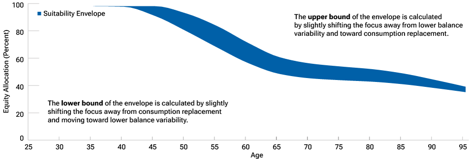
Source: T. Rowe Price. For illustrative purposes only. Not representative of an actual investment. This analysis contains information derived from a Monte Carlo simulation. This is not intended to be investment advice or a recommendation to take any particular investment action. See Additional Disclosures for more information.
This exercise enables plan sponsors to identify a glide path that is similar to the model’s baseline recommendation but that they may find more appropriate for their objectives.
Putting it all together
All else being equal, the presence of a DB plan should improve investors’ retirement income outlook. It implies that they will not require as much growth in their DC plan assets to meet their retirement income needs and thus can afford to reduce exposure to potential balance instability. The resulting impact on the appropriate glide path is to push the equity allocation downward.
However, all else is not always equal. There are multiple instances where a higher equity glide path may be appropriate despite the presence of a DB plan. For example, a plan sponsor might choose to focus more on the most vulnerable or DC‑reliant participants in their plan, who still may need more growth even with their defined benefits.
In this particular case, the DB plan gives the sponsor greater flexibility to focus on more vulnerable populations without disadvantaging those who are more financially secure because they are in a better position to absorb short‑term equity volatility due to the presence of the DB plan. In effect, the plan sponsor could be revealing one of two distinct preferences—either a greater preference for consumption vis‑à‑vis wealth, or a lower aversion to risk, or perhaps a combination of both.
The above example underpins our core belief that preferences matter. They also are the key to understanding our view that evaluating the implications of the presence of a DB plan for glide path design is not as simple as some prescribe. This is why we believe a “single” right answer does not exist. Accordingly, the goal of the Making the Benefit Connection series is to introduce readers to the full gamut of considerations involved in this decision and their various contours. We seek to provide plan sponsors with the tools to create a process for evaluating these considerations and make the best decision they can.
Conclusion
Our approach to glide path design focuses directly on measuring potential outcomes and responding to preferences, not on achieving an idealized, impersonal, overall asset allocation. Our glide path designs flow naturally from a utility model that we believe is both parsimonious and economically rigorous. In practice, this means that our equity weights are often higher than those in competing glide paths, although our nuanced approach makes direct comparisons difficult, in our view.
We have designed our glide path construction framework to identify a single glide path that we believe is appropriate for heterogenous populations. Beyond the inherent heterogeneity of individual preferences and demographics, and the potential for diverse macroeconomic scenarios to unfold, the presence of a DB plan adds a further degree of heterogeneity to the analysis.
As DC plans have grown in popularity, some plan sponsors have decided to limit access to their DB plans in multiple ways. Our perception is that many sponsors who have not done so yet are considering it. However, in our work we have found that, beyond making a few simple assumptions, relatively few plan sponsors are accounting for their DB plans—regardless of participant access—when assessing and selecting glide paths for their DC plans. We believe this oversight has the potential to lead to suboptimal choices that fall short of a glide path that is most appropriate for a plan’s objectives and preferences.
The third installment of the Making the Benefit Connection series examines the effect of frozen and closed plans on a DC plan glide path.
Important Information
This material is being furnished for general informational and/or marketing purposes only. The material does not constitute or undertake to give advice of any nature, including fiduciary investment advice. Prospective investors are recommended to seek independent legal, financial and tax advice before making any investment decision. T. Rowe Price group of companies including T. Rowe Price Associates, Inc. and/or its affiliates receive revenue from T. Rowe Price investment products and services. Past performance is no guarantee or a reliable indicator of future results.. The value of an investment and any income from it can go down as well as up. Investors may get back less than the amount invested.
The material does not constitute a distribution, an offer, an invitation, a personal or general recommendation or solicitation to sell or buy any securities in any jurisdiction or to conduct any particular investment activity. The material has not been reviewed by any regulatory authority in any jurisdiction.
Information and opinions presented have been obtained or derived from sources believed to be reliable and current; however, we cannot guarantee the sources’ accuracy or completeness. There is no guarantee that any forecasts made will come to pass. The views contained herein are as of the date written and are subject to change without notice; these views may differ from those of other T. Rowe Price group companies and/or associates. Under no circumstances should the material, in whole or in part, be copied or redistributed without consent from T. Rowe Price.
The material is not intended for use by persons in jurisdictions which prohibit or restrict the distribution of the material and in certain countries the material is provided upon specific request. It is not intended for distribution to retail investors in any jurisdiction.
USA—Issued in the USA by T. Rowe Price Associates, Inc., 100 East Pratt Street, Baltimore, MD, 21202, which is regulated by the U.S. Securities and Exchange Commission. For Institutional Investors only.
© 2024 T. Rowe Price. All Rights Reserved. T. ROWE PRICE, INVEST WITH CONFIDENCE, and the Bighorn Sheep design are, collectively and/or apart, trademarks of T. Rowe Price Group, Inc.
March 2024 / MULTI-ASSET INSIGHTS
