
March 2022 / RETIREMENT
When the Retirement Clock Gets Wound Forward
Glide path design should reflect possibility of early retirement.
Key Insights
- Many defined benefit plans allow or encourage early retirement by granting participants access to benefits prior to Social Security full retirement age.
- The decision to retire early can materially increase the amount of wealth needed to sustain income over a longer period.
- Sponsors evaluating their defined contribution glide paths should account for the wealth and early retirement incentives provided by a defined benefit plan.
Previously in our Benefit Connection series, we explored how the additional wealth provided by a defined benefit (DB) plan can impact the target date glide path in an accompanying defined contribution (DC) plan, particularly if the substitution effect isn’t considered.1 We showed how this additional wealth generally pushes down the equity allocation across most ages. However, we didn’t consider the impact that the presence of a DB plan might have on when participants choose to retire. We do so here.
Data from U.S. corporate pension plan regulatory filings suggest that participants who have DB plan benefits often retire earlier than the Social Security full retirement age, which is transitioning from age 66 to age 67 (Figure 1). This is particularly true when plans offer early retirement subsidies, which creates a retirement benefit that is more valuable than the actuarially reduced benefit.
Almost 90% of U.S. Corporate Plans Have an Average Retirement Age of 65 or Lower
(Fig. 1) Weighted average retirement ages for DB plans with 10+ participants

(Fig. 1) Weighted average retirement ages for DB plans with 10+ participants
Source: U.S. Employee Benefits Security Administration, 2020 Form 5500 dataset (n = 17,029). Data analysis by T. Rowe Price.
While aggregated U.S. public plan data are harder to come by, the typical design of many local government, firefighter, and law enforcement DB plans leads us to expect that the average retirement age for these participants is lower than the Social Security full retirement age, just as we see in the U.S. corporate sector. If a DB plan encourages employees to retire earlier than they otherwise would, the glide path for a companion DC plan’s target date offering should reflect this earlier transition from accumulation to decumulation.
Many DC plan glide paths, including the ones offered by T. Rowe Price in our flagship commingled vehicles, are built on the assumption that participants will retire at a specific age, typically 65. An earlier retirement date will impact postretirement wealth and spending in several ways for participants who have both DB and DC benefits.
- Most obviously, the DC asset accumulation phase will be shorter, while the decumulation phase will be longer.
- Any defined benefit that incorporates a service multiplier will provide less retirement income, reflecting the participant’s shorter career. Similarly, a cash balance plan participant retiring early would receive fewer pay credits.
- Even if the defined benefit does not directly depend on service years or pay credits, the benefit is likely to be reduced for an early retiree, due to actuarial equivalence plan provisions that adjust benefits lower to account for mortality and the time value of money, especially if the early retirement benefit is not subsidized.
- Early retirees also may have lower annual retirement liabilities compared with participants who retire at the normal age, depending on potential salary growth during their later working years.
Impact on glide path suitability
To assess how much glide paths should change to reflect lower retirement ages, we modeled four hypothetical scenarios, all of which are based on the baseline safe harbor DC plan that we have used throughout the Benefit Connection series:
- Baseline: The employer matches 100% of the first three percentage points of employee salary deferrals and 50% of the next two percentage points, for a maximum employer contribution of 4% of salary. There is no accompanying DB plan.
- Final average pay (FAP) plan: The same DC plan, paired with a final average pay DB plan that pays normal retirement benefits at the normal retirement date, equaling 1% x the average of the final five years of pay x years of service.
- FAP plan with early retirement: The same DC and final average pay DB plans described in scenario 2, but optimized for retirement at age 61 with a benefit that is actuarially equivalent to the normal retirement benefit.2
- FAP plan with subsidized early retirement: The same DC and final average pay DB plans assumed in scenarios 2 and 3, but optimized for retirement at age 61 with a benefit that is subsidized relative to the actuarially equivalent normal benefit.3
Not surprisingly, and consistent with the findings in the other papers in the Benefit Connection series, the addition of the FAP plan brought the hypothetical optimal glide path equity allocation down significantly throughout both the accumulation and decumulation phases (Figure 2). The largest disparity occurred in the peak earning ages for someone retiring at age 65. However, when we took the same DB plan and allowed a participant to retire at age 61 with an actuarially equivalent benefit, the impact on the hypothetical glide path equity allocation was much more muted (Figure 3).
The biggest difference in equity allocations between the FAP plan with early retirement (scenario 3) and the baseline scenario (i.e., a DC plan without a companion DB plan) occurred well into retirement and was only about eight percentage points in magnitude. The longer retirement period required significant DC plan portfolio growth throughout the accumulation phase in order to be sustainable.
By its very nature, the early retirement subsidy provided in scenario 4 increased retirement wealth, so we saw a two- to four-percentage-point reduction in the hypothetical optimal equity allocation throughout the glide path in comparison with the unsubsidized early retirement glide path in scenario 3. The impact of the subsidy was largest in the years right around retirement, since those were the years when the additional wealth from the subsidy would have been realized.
Conclusions
Early Retirement Brought Equity Up Toward Baseline Scenario
(Fig. 2) Hypothetical optimal glide path equity allocations
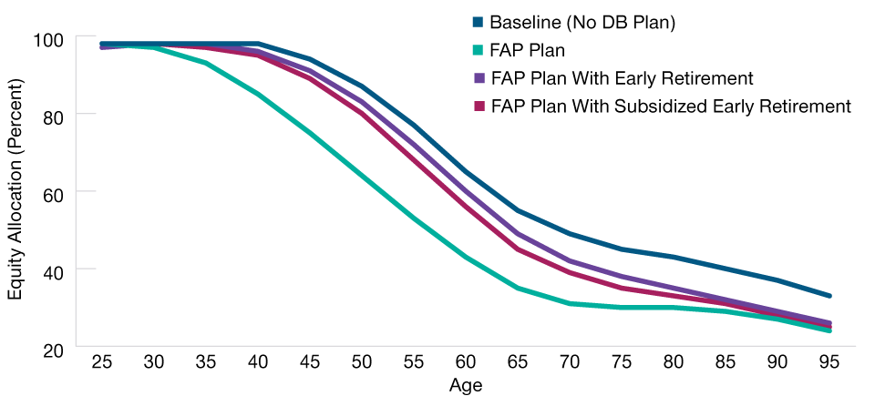
Source: U.S. Employee Benefits Security Administration, 2020 Form 5500 dataset (n = 17,029). Data analysis by T. Rowe Price. For illustrative purposes only. Not representative of an actual investment. This analysis contains information derived from a Monte Carlo simulation. This is not intended to be investment advice or a recommendation to take any particular investment action. See Appendix for more information.
While the addition of a DB plan to an existing DC plan can improve participants’ overall retirement wealth, if the existence of the DB plan encourages employees to retire early, there could be several offsetting factors that affect glide path design.
Early Retirement Significantly Offset DB Wealth Effect in Accumulation Phase
(Fig. 3) An unsubsidized FAP plan reduced equity by less than eight percentage points vs. baseline
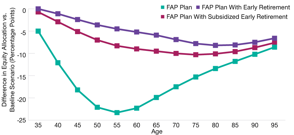
Source: T. Rowe Price.
For illustrative purposes only. Not representative of an actual investment. This analysis contains information derived from a Monte Carlo simulation. This is not intended to be investment advice or a recommendation to take any particular investment action. See Appendix for more information.
If their early-retirement DB benefits are unsubsidized, participants still will need significant equity exposure in their DC plans to sustain their longer retirement periods. In this case, the DB benefit would likely be lower due to both a shorter career service multiplier and a reduction to reflect the actuarial impact of mortality and the time value of money.
Even with a subsidy, the full wealth effect of having a DB plan is not realized for early retirees when compared with those who retire at a later retirement age. Higher equity allocations and investment returns would still be needed to support a longer decumulation horizon.
Important Information
This material is being furnished for general informational and/or marketing purposes only. The material does not constitute or undertake to give advice of any nature, including fiduciary investment advice. Prospective investors are recommended to seek independent legal, financial and tax advice before making any investment decision. T. Rowe Price group of companies including T. Rowe Price Associates, Inc. and/or its affiliates receive revenue from T. Rowe Price investment products and services. Past performance is no guarantee or a reliable indicator of future results.. The value of an investment and any income from it can go down as well as up. Investors may get back less than the amount invested.
The material does not constitute a distribution, an offer, an invitation, a personal or general recommendation or solicitation to sell or buy any securities in any jurisdiction or to conduct any particular investment activity. The material has not been reviewed by any regulatory authority in any jurisdiction.
Information and opinions presented have been obtained or derived from sources believed to be reliable and current; however, we cannot guarantee the sources’ accuracy or completeness. There is no guarantee that any forecasts made will come to pass. The views contained herein are as of the date written and are subject to change without notice; these views may differ from those of other T. Rowe Price group companies and/or associates. Under no circumstances should the material, in whole or in part, be copied or redistributed without consent from T. Rowe Price.
The material is not intended for use by persons in jurisdictions which prohibit or restrict the distribution of the material and in certain countries the material is provided upon specific request. It is not intended for distribution to retail investors in any jurisdiction.
USA—Issued in the USA by T. Rowe Price Associates, Inc., 100 East Pratt Street, Baltimore, MD, 21202, which is regulated by the U.S. Securities and Exchange Commission. For Institutional Investors only.
© 2024 T. Rowe Price. All Rights Reserved. T. ROWE PRICE, INVEST WITH CONFIDENCE, and the Bighorn Sheep design are, collectively and/or apart, trademarks of T. Rowe Price Group, Inc.
March 2022 / INVESTMENT INSIGHTS