Asset Allocation: Beyond Diversification

Our Global Multi-Asset team has received a growing number of requests from clients to talk about our views on strategic asset allocation (SAA), as opposed to the usual market outlook discussions popular at this time of year. A growing number of clients are rethinking portfolio construction given the paradigm shift from an environment of low interest rates and inflation to one of rising rates and higher inflation.

At a recent online event for Asian institutional clients, I spoke on this important topic. How does T. Rowe Price’s Global Multi-Asset team allocate portfolios across its USD 400 billion franchise¹ when the world is experiencing an abrupt paradigm shift from three decades of declining interest rates to a prolonged period of higher rates? In response to such a major structural shift, we believe that investors need to rethink portfolio construction from a strategic or long-term perspective.²

In today’s tough markets, the initial response of investors might be to increase the time and resources spent on developing their short-term market views and projections. This is understandable. However, the long-term asset allocation implications of the shift to higher rates arguably matters more. There is considerable empirical evidence to suggest that strategic asset allocations can drive long-term returns and risks more than any other investment decision.

Long-Term Returns and Valuations

Strategic asset allocation usually begins with assumptions for the long-term returns to stocks and bonds. While forecasting asset returns is always difficult, it is possible to arrive at some working assumptions that have proved to be useful in practice.

Turning to Figure 1, the chart on the left shows the relationship between the Shiller cyclically adjusted price earnings (or CAPE) ratio and subsequent 10-year equity returns. The CAPE is simply the ratio of the S&P 500 Index’s price to trailing 10-year earnings, adjusted for inflation, which smooths the earnings cycle. The correlation is 54%, which is not bad for this type of relationship. It tells us that what you pay for stocks, in terms of multiple of earnings, matters a lot for subsequent long-term returns. When markets are expensive, subsequent returns tend to be lower, as evidenced by the downward slope of the regression line. And vice versa when markets are cheap.

The middle panel of Figure 1 shows an alternative comparison between equity returns and valuations using the current trailing 12-month earnings yield (the inverse of the PE ratio), sometimes referred to as the “Siegel” model. The fit is different, but also quite good. Interestingly, the correlation is about the same, which suggests that there is nothing particularly magical about the CAPE approach. The first two panels of Figure 1 simply tell us that if you have a long investment horizon, then you should pay attention to starting valuation levels. Buy low; sell high!

Turning to bonds, the right-hand panel of Figure 1 plots the starting or opening yield of a 10-year U.S. Treasury against the long-term return from holding the bond to maturity. In this case, the fit is remarkable, with a correlation of 91%. The starting yield of a long-term government bond is a good predictor of the subsequent return for a bond held to maturity. Besides return predictability, there is an important takeaway if you are a long-term investor, such as in a pension or insurance fund. Rising rates are good news for long-term bond investors, because when yields rise, the long-term expected return on their bonds held to maturity increases.

Expected 10-Year Returns in 2022

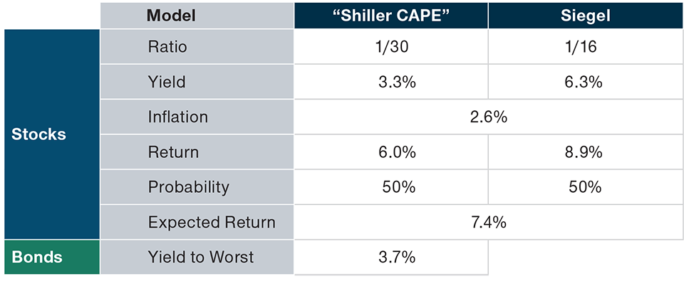
What can the historical relationships for stocks and bonds shown in Figure 1 tell us about long-term expected returns from where we stand today? The simplest way to convert equity valuations into an expected return is to invert the P/E ratio. This gives you the earnings yield, which from Figure 1 is a reasonably good predictor of long-term equity returns. Taking the U.S. as an example, Figure 2 shows earnings yields for the CAPE and Siegel models of 3.3% and 6.3%, respectively, which are real returns. To make them comparable with a nominal expected bond return, we need to add on an estimate for inflation. Our inflation adjustment of 2.6% is close to the 10-year break-even inflation as of August 2022. This gives expected nominal equity returns of 6.0% for the CAPE model and 8.9% for the Siegel model.

Taking an equal-weighted average of the two methods gives us an expected equity return of 7.4% (the Siegel model is arguably more realistic over shorter- to medium-term horizons, while the CAPE favors the longer term). For bonds, the yield on the Bloomberg Global Aggregate Bond Index at the time of writing was 3.7%, so from Figure 1 we take that as our nominal expected total return from government bonds over the next 10 years.

Expected Returns and Portfolio Construction

Now, there are more sophisticated ways to forecast long-term returns than the simple valuation-based methods that we have employed above. Nevertheless, there are some useful lessons for portfolio construction that follow on from our analysis.

First, despite higher rates, today’s investors face the challenge of significantly lower future returns than in the past decade. Figure 3 shows that historic 30-year returns have averaged around 10% for stocks and 5.9% for bonds. These are significantly higher than our projected future 10-year returns of 7.4% and 3.7%. For the 60/40 traditional balanced portfolio, we could take a nominal return close to 6.0% as a reasonable estimate of future returns, or (0.6 x 7.4%) + (0.4 x 3.7%).

The portfolio allocation diagram on the left-hand side of Figure 3 shows that over the last 30 years, bond returns were so good (5.9% annualized) that you only needed to add a little boost (2% to 3% allocation) from stocks to get to a 6% target expected return for the hypothetical portfolio. But from where we are today, if you wanted to achieve an expected return of 6% over the next 10 years, you would need to put over 60% of your portfolio into stocks (right-hand asset allocation, Figure 3).

A 6% nominal target return is not actually that high. If an investor wanted to achieve more than that, they would have to crank up the risk level. That could be a mistake if the investor takes on more risk than they can bear in an effort to “stretch” for higher returns. So, one important lesson we can draw is that it would be wise for investors to lower their expectations. If you’re involved in SAA and work with clients, that’s probably the most important thing you can tell them: Lower your expectations relative to history because the world has changed and high returns are harder to come by today.

Risk Considerations and “Black Swan” Events

What about the risk side? An important issue in risk management is whether the correlations between assets remain stable over time. They do not. I once coauthored a paper titled “The Myth of Diversification,” explaining what most investors know intuitively: that risk assets become extremely correlated whenever markets sell off, i.e., there is no place to hide. In that paper, we also explained that not only are correlations very high during a market crisis, but they also tend to be very low during market rallies, in good times. That’s exactly the opposite of what we want to see as investors. This is not an argument against diversification—far from it. Instead, I’m arguing that diversification must account for exposure to losses during market crises, rather than long-term averages.

Another important topic in risk management is the presence of so-called black swan, or very rare, events. Although this is a well-known issue in finance, I think many investors are still inclined to underestimate the importance of “fat tails,” or extreme events. In a 2001 paper, Andrew Lo presented a fascinating case study on this issue. Based on monthly data from January 1992 to December 1999, he simulated an investment strategy that required no investment skill whatsoever. No analysis, no foresight, no judgment.

Despite its simplicity, in Lo’s backtest, the strategy doubled the Sharpe ratio of the S&P 500 from 0.98 to 1.94. Can you guess what the strategy was? In the simulation, Lo sold out-of-the-money put options on the S&P 500. Essentially, the strategy sold insurance. It loaded up on tail risks. It picked up pennies in front of a steamroller.³ Many risk premia, especially those focused on carry, credit, volatility, or liquidity premia, are in effect short an option.

Tail events also have major implications for how we should think about diversification. The important takeaway here is that investors should be suspicious of estimating risk based purely on traditional measures of volatility. It follows that investors should also be suspicious of Sharpe ratios too. Instead, we recommend that they try to equip themselves with downside risk measures combined with scenario analysis tools.

Optimization

Some investors might be comfortable using optimization tools to allocate assets in a way that maximizes the expected return while controlling explicitly for risk. But are such tools useful in practice as opposed to in an academic course on finance theory? I was at a quantitative research conference once when somebody asked whether optimizers were of any use, since they required inputs, in particular, expected returns, were too difficult to estimate. The presenter answered the question with something I will always remember: “If you don’t think you can estimate expected returns, then you shouldn’t be in the investment business.” Investing is, indeed, mostly about forecasting returns. Even investors who do not formulate expected returns as a precise number must still make implicit forecasts when they allocate assets. So the difficulty of forecasting returns is no excuse not to use optimizers.

Related to this critique, there is a popular myth—propagated by some academics -—that equal-weighting portfolios is better than optimizing portfolios. I strongly disagree. In a paper I coauthored in the Financial Analysts Journal, we showed that if you use sensible inputs in your asset allocation process, then you can add value with optimization.

 

Modernizing the 60/40 Portfolio

A key conclusion from our analysis above is that future long-term returns are likely to be significantly lower than what investors have enjoyed in the past. Interest rates are rising, and inflation risk has become more important. Thoughtful risk management, more than ever, needs to consider ‘black swan’ risks and the failure of diversification when we need it the most. What does this mean, say, for how we should rethink the typical 60% stocks, 40% bonds balanced portfolio? Figure 4 shows a modernized 60/40 model portfolio that seeks to improve diversification by adding more asset classes.

Of the 40% traditional bond allocation, 12% is switched into liquid alternatives. Also within bonds, the portfolio employs a barbell structure between long maturity bonds (a capital-efficient way of hedging against growth shocks but not interest rate shocks) and diversified credit instruments, such as emerging market bonds, high yield bonds, and bank loans.

Within equities, our modernized 60/40 model portfolio tilts toward high alpha diversifiers, such as small- and mid-cap stocks and emerging market stocks. There is also a 10% risk-managed equity sleeve, which aims to make up for the loss of diversification from government bonds during the kind of interest rate and inflation shocks that we have encountered in 2022.

If you would like to learn more about this type of highly diversified model portfolio designed to suit today’s challenging environment, please contact your T. Rowe Price representative, and tell them Sébastien Page sent you!