On Retirement
Plan Sponsor, Plan Sponsor, Make Me a Match
Savings behavior impacts glide paths more than DC match formulas.
Justin Harvey, ASA, CFA Head of Analysis, Multi‑Asset Solutions
Adam Langer, CFA Senior Quantitative Investment Analyst
Key Insights
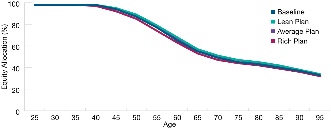
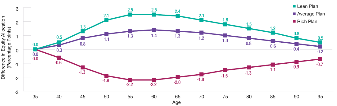
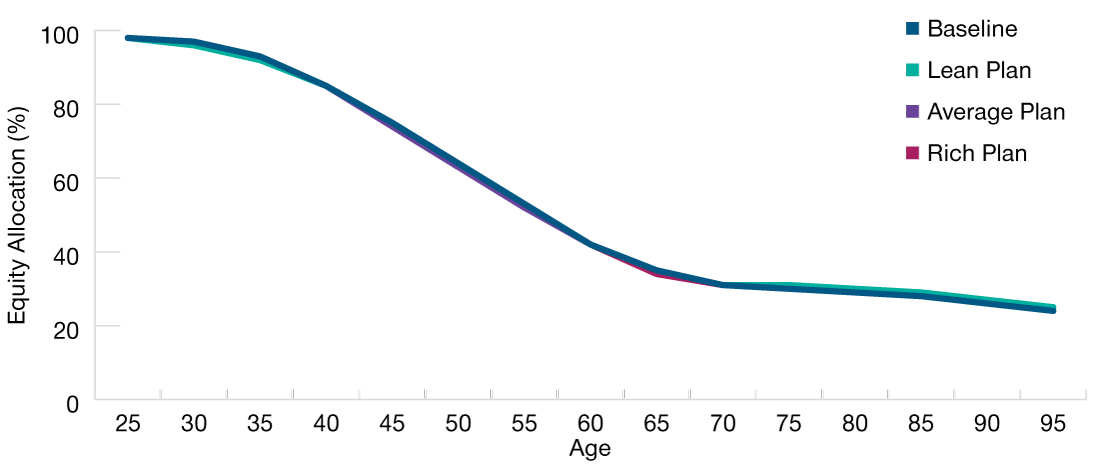
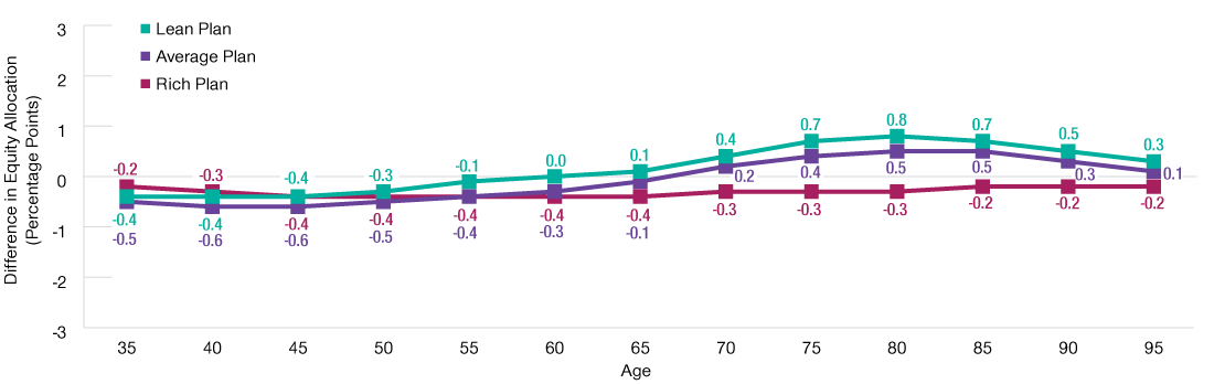
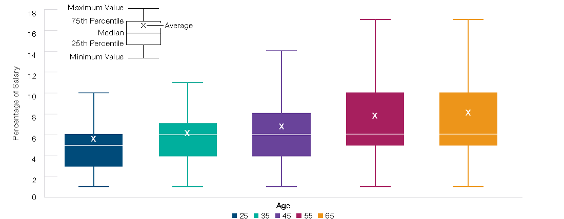
  • Our modeling work found that participant savings behavior had a greater impact on glide path design than employer match generosity did.
  • The richness of the match formula shifted the optimal glide path equity allocation by less than 5% at all ages, even in the absence of a defined benefit plan.
  • These findings support the idea that participants ultimately own their outcomes when their retirements are supported primarily by defined contribution plans.

The preceding paper in our Benefit Connection series explored how different defined benefit (DB) designs can impact the target date glide path in an accompanying defined contribution (DC) plan. We showed how cost‑of‑living adjustments, lump‑sum availability, and benefit accrual patterns all can materially impact glide path design in various ways.1

While DC plans also may include a wide array of design features—such as auto‑enrollment, the inclusion of a qualified default investment alternative (QDIA), and the specific investment lineup offered, just to name a few—the employer match is the feature we are most frequently asked about in relation to glide path appropriateness.

Employer contributions also can take many forms, but the advantage of a match formula is that it tends to promote better participant savings behavior and thus may result in higher account balances over time. Matching is also is the most common contribution feature for the plans on T. Rowe Price’s recordkeeping platform. In this paper, we review how three different employer match formulas influenced the optimal glide path design in our modeling analysis.2

Plan Design Assessment

To assess how much glide paths should change based on various match formulas, we modeled four hypothetical plan designs, including the baseline safe harbor plan that we have used so far in the Benefit Connection series.

1. Baseline: The employer matches 100% of the first three percentage points of employee salary deferrals and 50% of the next two percentage points, for a maximum employer contribution of 4% of salary.

2. Lean: The employer matches 50% of the first four percentage points in salary deferrals, for a maximum employer contribution of 2% of salary.

3. Average: The employer matches 50% of the first six percentage points in salary deferrals, for a maximum employer contribution of 3% of salary.

4. Rich: The employer matches 100% of the first six percentage points in salary deferrals, for a maximum employer contribution of 6% of salary.

The lean, average, and rich designs collectively comprised nearly half of the match formulas offered by the plans on our recordkeeping platform, with the average formula being the most common. We believe these designs represent a reasonable range in employer generosity—while acknowledging that there are match formulas that are leaner or richer than the ones modeled in our analysis.

2.5 Percentage Points
Maximum difference in glide path equity allocations relative to the baseline plan, based on the  assumed employer match formula.

Figure 1 shows the hypothetical glide paths that our model identified as optimal for the four designs. Equity allocations in the lean and average glide paths were slightly above the baseline design. However, the maximum difference at any age was only 2.5 percentage points or less (Figure 2). The rich glide path featured slightly lower equity levels at age 40 and above, reflecting less need for participants in those plans to assume market risk to meet their retirement income targets, given their higher overall savings.

Match Generosity Had Minimal Impact on Glide Path Equity

(Fig. 1) Glide paths for hypothetical DC plans with varying match formulas

Glide paths for hypothetical DC plans with varying match formulas

Source: T. Rowe Price.

For illustrative purposes only. Not representative of an actual investment or T. Rowe Price product. This analysis contains information derived from a Monte Carlo simulation. See Appendix for for additional important disclosures.

Only Minor Variations in Optimal Glide Path Equity Levels

(Fig. 2) Change in hypothetical equity allocations relative to baseline plan

Change in hypothetical equity allocations relative to baseline plan

Source: T. Rowe Price.

For illustrative purposes only. Not representative of an actual investment or T. Rowe Price product. This analysis contains information derived from a Monte Carlo simulation. See Appendix for for additional important disclosures.

Overall, the maximum equity allocation difference (between the rich and the lean glide paths) was less than five percentage points at all ages. These relatively minor differences may be surprising, given that the match formula typically has the most impact on the cost of a plan. However, as we shall see, it does not necessarily have a major influence on glide path appropriateness when the match is altered in isolation.3

In our models, the impact of different match formulas on the optimal glide path was even further muted when the DC plan was paired with an accompanying final average pay DB plan (Figures 3 and 4), because the participant income provided by the DB plan made the employer’s DC plan contributions an even smaller share of total retirement wealth.

This result only would have been reinforced if our model had reflected the reality that plan sponsors seeking to preserve liquidity have greater discretion to suspend their DC match formulas than to avoid the regulatory required minimum contributions for corporate DB plans or legislated funding requirements for some public DB plans. Throughout the 2008–2009 global financial crisis and more recently during the COVID‑19 pandemic, we saw several companies take advantage of this flexibility.

Even when we applied the same DC match formula across the entire length of an employee’s career, it still did not materially affect the optimal glide path in our model. A temporary suspension in the employer match would have reduced this impact even further.

Even Less Impact When Paired With a Hypothetical DB Plan

(Fig. 3) Glide paths for hypothetical DC plans with varying match formulas

Glide paths for hypothetical DC plans with varying match formulas

Source: T. Rowe Price.

For illustrative purposes only. Not representative of an actual investment or T. Rowe Price product. This analysis contains information derived from a Monte Carlo simulation. See Appendix for for additional important disclosures.

DB Plan Income Further Reduced Variations in Glide Path Equity

(Fig. 4) Change in hypothetical equity allocations relative to baseline plan

Change in hypothetical equity allocations relative to baseline plan

Source: T. Rowe Price.

For illustrative purposes only. Not representative of an actual investment or T. Rowe Price product. This analysis contains information derived from a Monte Carlo simulation. See Appendix for for additional important disclosures.

Why the Surprising Results?

T. Rowe Price recordkeeping data indicate that most plan participants respond rationally to incentives over their careers, meaning they start by saving at least as much as is required to maximize the employer match and then increase their salary deferrals as they age. Increased plan use of auto‑enrollment and auto‑escalation features probably has helped reinforce this behavior, which also is incorporated in our analysis (Figure 5).

Recently, we’ve seen renewed sponsor interest in further encouraging participant savings by stretching a lower match percentage to cover a higher percentage of salary deferral—for example, by offering to match 50% of the first 8% of salary rather than 100% of the first 4%.

Match formula design changes, in isolation, seemed to have minimal impact on the optimal glide path equity allocations indicated in our model. While we did not explicitly model the impact of different match designs on employee savings behavior, this is an area of research that we think warrants further exploration—particularly the impact of match formulas that require employees to defer a higher salary percentage to receive the full match.

In the population set we assumed for this paper—based on data from T. Rowe Price’s recordkeeping platform as of 2020—70% of participants started out saving at least 4% of salary and 50% started out saving at least 5%. By age 30, more than 50% of participants were deferring at least 6% of salary, a level that maximized the employer contributions in all the plans we modeled.

In the designs we modeled, the difference in the maximum employer contribution between the rich and lean plans was only 4% of salary (ranging from 2% to 6%), whereas the average participant deferral varied between 5.6% and 8.1% of salary, depending on age.4 Viewed through this lens, it’s not surprising that match generosity had a relatively small impact on optimal equity levels in the hypothetical plans we modeled. Most participants were deferring more than the employer match over most of their careers. This suggests that even when a plan sponsor cannot afford a generous match, there still may be opportunities to improve retirement outcomes by implementing auto features and incentivizing participant savings behavior.5

Higher Savings Reduced the Impact of Match Generosity

(Fig. 5) Distribution of salary deferral rates by age, 10,000 simulations

Distribution of salary deferral rates by age, 10,000 simulations

Source: T. Rowe Price.

For illustrative purposes only. Not representative of an actual investment or T. Rowe Price product. This analysis contains information derived from a Monte Carlo simulation. See Appendix for for additional important disclosures.

Conclusions

While employers can prioritize matching contributions over other forms of compensation, our analysis indicates that participant behavior ultimately has the greatest impact on glide path equity allocations and on retirement readiness. Our recordkeeping data indicate that DC plan sponsors are having some success convincing participants of the importance of increasing savings, which ultimately reduces the standalone impact of the employer contribution on glide path design.

"While employers can prioritize matching contributions... our analysis indicates that participant behavior ultimately has the greatest impact on glide path equity allocations and on retirement readiness."

Appendix

Key Modeling Plan Design Parameters

Hypothetical DC plans: Our baseline assumption was a safe harbor plan design with the employer matching up to 100% of the first three percentage points of salary deferrals and 50% of the next two percentage points. We also modeled “lean,” “average,” and “rich” plan designs based on the employer match formulas most frequently used by the plans on T. Rowe Price’s DC recordkeeping platform. We assumed all contributions were pretax and that contributions increased over time according to our proprietary deferral rate growth model.

Hypothetical DB plan: A final average pay plan that paid a single life annuity with the following benefit formula: normal retirement benefit at normal retirement date equaled 1% x the average of the final five years of pay x years of service.

Demographic analysis: We assumed that participant incomes grew in line with a proprietary salary growth model calibrated on our recordkeeping platform. Participants were assumed to retire at age 65 and to begin withdrawing income to support a steady, inflation‑adjusted level of spending over retirement.

Projections or other information generated regarding the likelihood of certain outcomes are not guarantees of future results. This analysis was based on assumptions, and there can be no assurance that the projected results will be achieved or sustained. Actual results will vary, and such results may be better or worse than the assumed scenarios.

Get the full story.

We’re ready to share our latest thinking, but industry regulations require you to register or sign in to continue reading this article. Thank you for understanding.

Just one more step.

To continue, you are required to read and accept our Terms & Conditions. Thank you for understanding.

1 Justin Harvey and Adam Langer. “The Importance of Defined Benefit Plan Design” (2021). The impact of pairing various DB plan designs with an existing DC plan varied the optimal equity level in the glide path by as much as 31 percentage points in the designs we modeled. We also found that DB plan eligibility and the amount of wealth provided by that plan both needed to be considered when evaluating glide paths.

2 For the details of our modeling methodology, please see the Appendix.

3 Assuming employee deferral levels are held constant for all match formulas.

4 The combination of employer matching contributions and participant deferrals brought total savings closer to the 15% of salary that we believe is appropriate for most participants. See Judith Ward. “Reasons Why You Should Aim to Save 15% for Retirement” (2021), and Roger Young. “You’re Age 35, 50, or 60: How Much Should You Have Saved for Retirement by Now?” (2021).

5 Joshua Dietch and Taha Choukhmane. “Auto‑enrollment’s Long‑Term Effect on Retirement Saving” (2019).


Additional Disclosure

Monte Carlo simulations model future uncertainty. In contrast to tools generating average outcomes, Monte Carlo analyses produce outcome ranges based on probability—thus incorporating future uncertainty.

Material Assumptions include:

  • Underlying economic and behavioral inputs, including savings rates and cash flows, are generated from a structural model built up from factors relating to both financial markets and the broad economy as well as data calibrated based on T. Rowe Price’s recordkeeping platform’s participant population.
  • The mortality weighting is sourced from the Society of Actuaries. Retirement age is assumed to be 65 years old.

Material Limitations include:

  • The analysis relies on assumptions, combined with a return model that generates a wide range of possible return scenarios from these assumptions. Despite our best efforts, there is no certainty that the assumptions and the model will accurately predict asset class return ranges going forward. As a consequence, the results of the analysis should be viewed as approximations, and users should allow a margin for error and not place too much reliance on the apparent precision of the results.
  • Users should also keep in mind that seemingly small changes in input parameters, including the initial values for the underlying factors, may have a significant impact on results, and this (as well as mere passage of time) may lead to considerable variation in results for repeat users.
  • Extreme market movements may occur more often than in the model.
  • Market crises can cause asset classes to perform similarly, lowering the accuracy of our projected return assumptions, and diminishing the benefits of diversification (that is, of using many different asset classes) in ways not captured by the analysis. As a result, returns actually experienced by the investor may be more volatile than projected in our analysis.
  • Asset class dynamics, including, but not limited to, risk, return, and the duration of “bull” and “bear” markets, can differ than those in the modeled scenarios.
  • The analysis does not use all asset classes. Other asset classes may be similar or superior to those used.
  • Fees and transaction costs are not taken into account.
  • The analysis models asset classes, not investment products. As a result, the actual experience of an investor in a given investment product may differ from the range of projections generated by the simulation, even if the broad asset allocation of the investment product is similar to the one being modeled. Possible reasons for divergence include, but are not limited to, active management by the manager of the investment product. Active management for any particular investment product—the selection of a portfolio of individual securities that differs from the broad asset classes modeled in this analysis—can lead to the investment product having higher or lower returns than the range of projections in this analysis.

Modeling Assumptions:

  • The primary asset classes used for this analysis are stocks and bonds. An effectively diversified portfolio theoretically involves all investable asset classes including stocks, bonds, real estate, foreign investments, commodities, precious metals, currencies, and others. Since it is unlikely that investors will own all of these assets, we selected the ones we believed to be the most appropriate for long-term investors.
  • The analysis includes 10,000 scenarios. Withdrawals are made annually at the beginning of each year.
  • IMPORTANT: The projections or other information generated by T. Rowe Price regarding the likelihood of various investment outcomes are hypothetical in nature, do not reflect actual investment results, and are not guarantees of future results. The simulations are based on assumptions. There can be no assurance that the projected or simulated results will be achieved or sustained. The charts present only a range of possible outcomes. Actual results will vary with each use and over time, and such results may be better or worse than the simulated scenarios. Clients should be aware that the potential for loss (or gain) may be greater than demonstrated in the simulations.
  • The results are not predictions, but they should be viewed as reasonable estimates.

Important Information

This material is provided for informational purposes only and is not intended to be investment advice or a recommendation to take any particular investment action. Prospective investors are recommended to seek independent legal, financial and tax advice before making any investment decision. This material does not provide fiduciary recommendations concerning investments or investment management.

The views contained herein are those of the authors as of February 2022 and are subject to change without notice; these views may differ from those of other T. Rowe Price associates.

This information is not intended to reflect a current or past recommendation concerning investments, investment strategies, or account types, advice of any kind, or a solicitation of an offer to buy or sell any securities or investment services. The opinions and commentary provided do not take into account the investment objectives or financial situation of any particular investor or class of investor. Please consider your own circumstances before making an investment decision.

Information contained herein is based upon sources we consider to be reliable; we do not, however, guarantee its accuracy.

Past performance is not a reliable indicator of future performance. All investments are subject to market risk, including the possible loss of principal. All charts and tables are shown for illustrative purposes only.

T. Rowe Price Investment Services, Inc., distributor, and T. Rowe Price Associates, Inc., investment advisor. For Institutional Investors Only.

© 2022 T. Rowe Price. All Rights Reserved. T. ROWE PRICE, INVEST WITH CONFIDENCE, and the Bighorn Sheep design are, collectively and/or apart, trademarks of T. Rowe Price Group, Inc.

Preferred Website

Do you want to go directly to the Financial Advisors/Intermediaries site when you visit troweprice.com ?

You are currently logged in to multiple T. Rowe Price websites.

You will need to log out below and log back in with your Advisor Dashboard credentials.