There are considerations that DC plan sponsors face when they want to optimize outcomes holistically across their retirement benefit offerings, including their defined benefit plan. DB plans encompass more structures than the common perception of a fixed dollar pension payable for life.
In this fifth installment of our Making the Benefit Connection series, we expand the notion of defined benefits to cover more of the category space. To this end, we used our proprietary models to construct a collection of hypothetical DC glide paths designed to be optimal complements for DB plans featuring varying benefit levels and payment patterns.
We used scenario analysis to compare these complementary glide paths across several features, including their shape and our full suite of metrics. This allowed us to explore the impact that the specific structure of a sponsor’s DB benefits can have on the characteristics of an accompanying DC glide path.1
Our results highlight the fact that it is a critical oversimplification to assume that different DB plan structures will influence the glide path for a companion DC plan in essentially the same way. In reality, the type of plan and its structural features—such as the form of payment, the accrual formula, and the inclusion or absence of cost-of-living indexing—can have a major impact on the level and slope of equity exposure in the glide path design.
Representative Plan Designs and Considerations
Up to this point in our series, we have assumed that defined benefit plans adhere to a structure like that of a fixed annuity. More specifically, we’ve assumed that payments are derived via a benefit formula incorporating tenure and salary:
Normal retirement benefit at normal retirement date = 1% x average of final five years of pay x years of service.
Traditionally, this type of final average pay (FAP) plan was common in corporate plans. Many sponsors understand that they can, for example, provide richer benefits by offering a replacement multiplier greater than 1% or provide lower-valued benefits (the more common trend recently) by considering the career salary average rather than the final five years, by capping the years of tenure used in the benefit calculation, or simply by reducing the multiplier.
Other changes have had more profound impacts. For example, like Social Security benefits, a defined benefit can include a cost-of-living adjustment (COLA) to attempt to maintain the real value of the payout over time. This is a more common feature in public pension plans. Historically, equity has often been considered a hedge against inflation in DC plans. But if an inflation hedge is built directly into the in-plan source of guaranteed income, DC plan participants may not need as much equity in their glide paths to perform this function, allowing sponsors to try to reduce balance variability by lowering the allocation to equity.
Cash balance (CB) plans, which often offer participants lump-sum options at retirement, have an entirely different benefit accrual and payout structure than their FAP counterparts. During employment, the plan sponsor issues credits to the employee, who accumulates a notional account balance.
There are two types of credits common to these plans: pay credits determined by a predefined formula, and interest credits, which often have an annually changing yield or investment return that determines the size of the credit.
Since the balance in a CB plan often acts like an allocation to low-risk fixed income assets during the benefit accrual phase, a participant’s remaining wealth held in a DC plan potentially could be invested in assets with a higher growth orientation than would be the case for a participant with an FAP plan.
Since most employees do take lump-sum benefits when offered, our analysis assumed that once a cash balance benefit had been paid, it was invested and allocated according to the accompanying DC glide path.2 Further details of the assumptions behind our cash balance plan example can be found in the appendix.
Different DB Plan Structures May Have Different Impacts
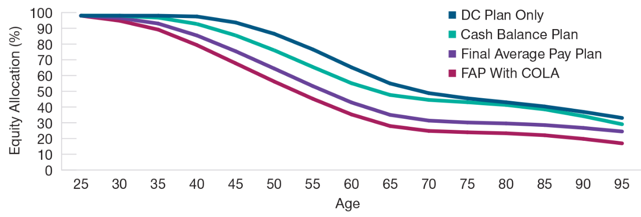
(Fig. 1) Glide paths for a hypothetical DC plan only vs. DC plan + various DB types
Glide Path Comparison
Figure 1 shows the plots of the optimal hypothetical glide paths calculated by our model for the baseline case of a standalone DC plan, and for the same DC plan design accompanied by examples of three different DB designs:
1. fixed yearly benefits based on a final average pay formula;
2. the same FAP plan with a COLA indexed to the U.S. Consumer Price Index with a 0% floor;
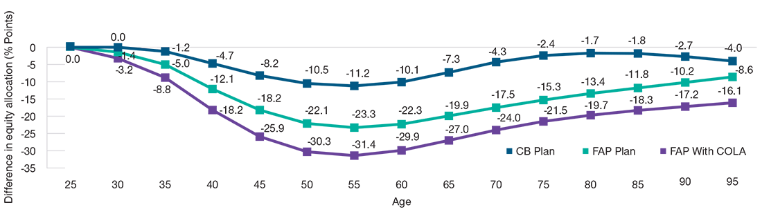
Figure 2 shows the relative differences in equity allocation at various points along these glide paths with respect to the baseline case of a hypothetical optimal glide path without an accompanying DB plan.
In our simulations, the CB plan indeed acted like a low-risk asset, resulting in higher optimal equity levels in the glide path for the accompanying DC plan during working years compared with the FAP plan and significantly higher equity exposure during retirement. This is because the lump-sum infusion of cash from the CB benefit had to continue to work hard during retirement to maintain preretirement consumption levels in the absence of guaranteed payments. In fact, in our simulations, the glide path for a DC plan accompanied by a CB plan that paid out in lump sums looked quite similar to the glide path for DC participants who did not have access to a DB plan after retirement.
Our assumed FAP plan with a COLA was, by explicit design, richer than a non-indexed FAP plan (whereas our CB plan was designed to be roughly cost and benefit equivalent to the non-indexed FAP plan). For the FAP plan with COLA, as for the non-indexed FAP, the resulting lower-equity glide path was an example of what we call the wealth effect. In short, since wealth is one source of utility in our model, having the added wealth from a DB plan led our model to decide that there was less need for utility from DC plan-supported consumption, allowing the DC plan to reduce risk and still achieve a good outcome, in our view.
However, the optimal glide path for an FAP plan with a COLA was even steeper during the working years because not as much real growth was needed from equities, thanks to the inflation hedge provided by the indexed DB benefit. Consequently, under our assumed preferences, the model lowered glide path equity levels in an effort to reduce risk and maintain utility from wealth. Meanwhile, the DB pension payments, in addition to Social Security benefits, provided consumption-based utility.
Optimal Equity Levels Can Vary Widely
(Fig. 2) Percentage point changes in glide path equity relative to a DC plan only baseline
Consumption Comparison
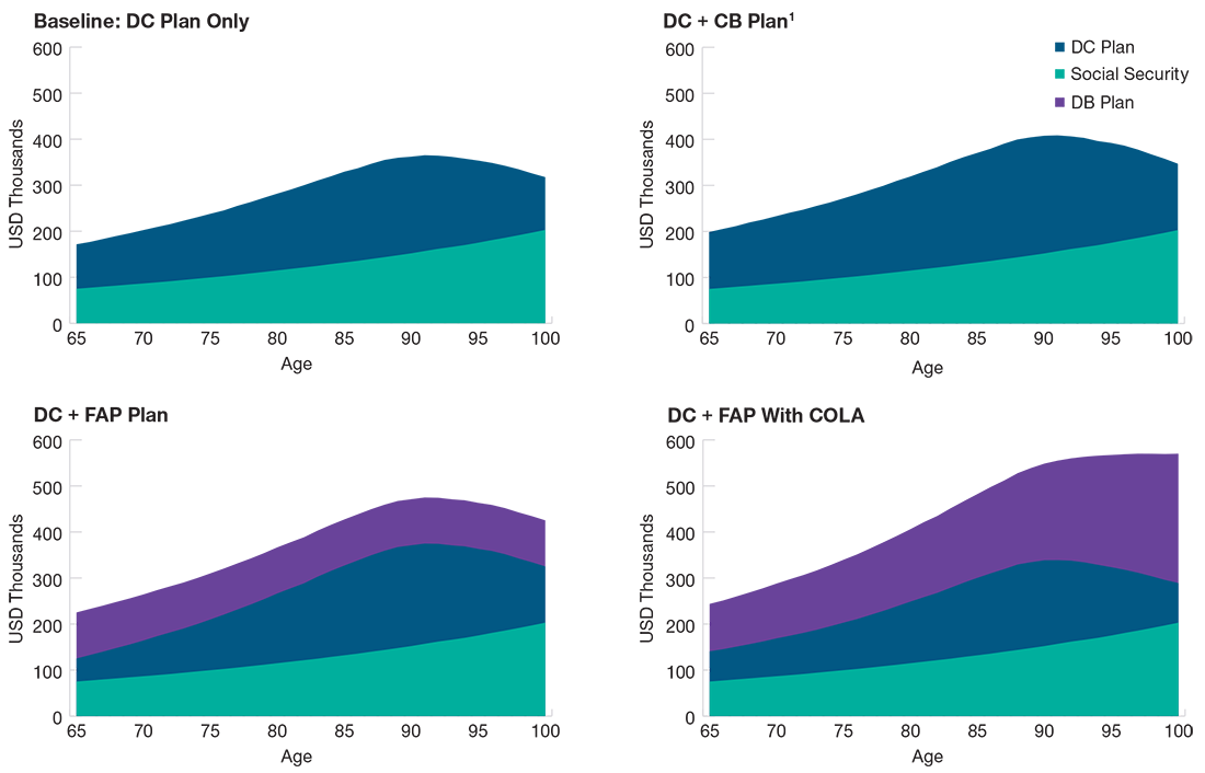
Consumption during retirement is not limited to the sum of Social Security and pension payments, but having both sources of income—each including its own method of real income replacement—can significantly reduce withdrawals from savings, represented here by the DC plan.
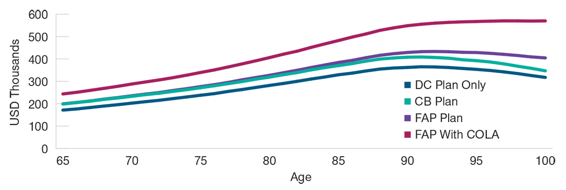
Figure 3 shows the median level of total consumption supported by each plan. Understanding the sources of consumption (shown here as median results from a broader Monte Carlo simulation) helped inform why the glide path shapes in Figure 3 differed, particularly after retirement. Figure 4 shows the sources of the consumption totals.
Notice that the consumption levels supported by the CB plan dropped most quickly after age 90, when they started to diverge noticeably from those provided by the non-indexed FAP plan. This is because the dwindling balance in the CB plan could not keep pace with the continued guaranteed payments in the FAP plan.
In the baseline case where there was no companion DB plan, the significantly higher equity allocation in the glide path throughout the accumulation phase provided a sufficient cushion, at the median, to meet consumption needs. In the simulations that included either a non-indexed FAP plan or an FAP with COLA, the guaranteed income streams alleviated the burden on savings, supporting consumption late into life.
FAP Plans May Support Higher Retirement Consumption
(Fig. 3) Median consumption support from a hypothetical DC plan only vs. DC plan + various DB structures
Consumption Is Supported by Various Plan Design Combinations
(Fig. 4) Consumption sources for a hypothetical DC plan only and a DC plan + various DB structures
Sensitivity to Inputs
Under our standard assumptions, the structure of a DB plan is an important consideration in determining an optimal glide path. These assumptions represent what we believe are reasonable sponsor goals, participant preferences, and demographic characteristics. However, we realize that it is unlikely that a specific plan sponsor will map to all of these exact assumptions. This being the case, we wanted to investigate what happened to the DB plan’s effect on the glide path when we modified certain assumptions. Specifically, we wanted to know if the results shown in Figures 1 and 2 still persisted.
In other words, were the optimal glide paths in our scenarios still as dependent on DB plan structure if we assumed that plan sponsors had different preferences than those incorporated in our original assumptions?
An important feature of our model is its explicit, numerical representations of plan sponsor goals for their DC plan. One such goal is setting the relative importance of consumption versus wealth. At the plan level, this manifests as a parameter in the model that can seek to limit exposure to market fluctuations in an effort to reduce balance variability over time. However, lower potential exposure to market fluctuations comes at the cost of an overall lower expected level of consumption over the long term. Alternatively, the model can seek higher growth in order to maintain higher consumption, at the risk of exposing participants to higher balance variability in the short term.
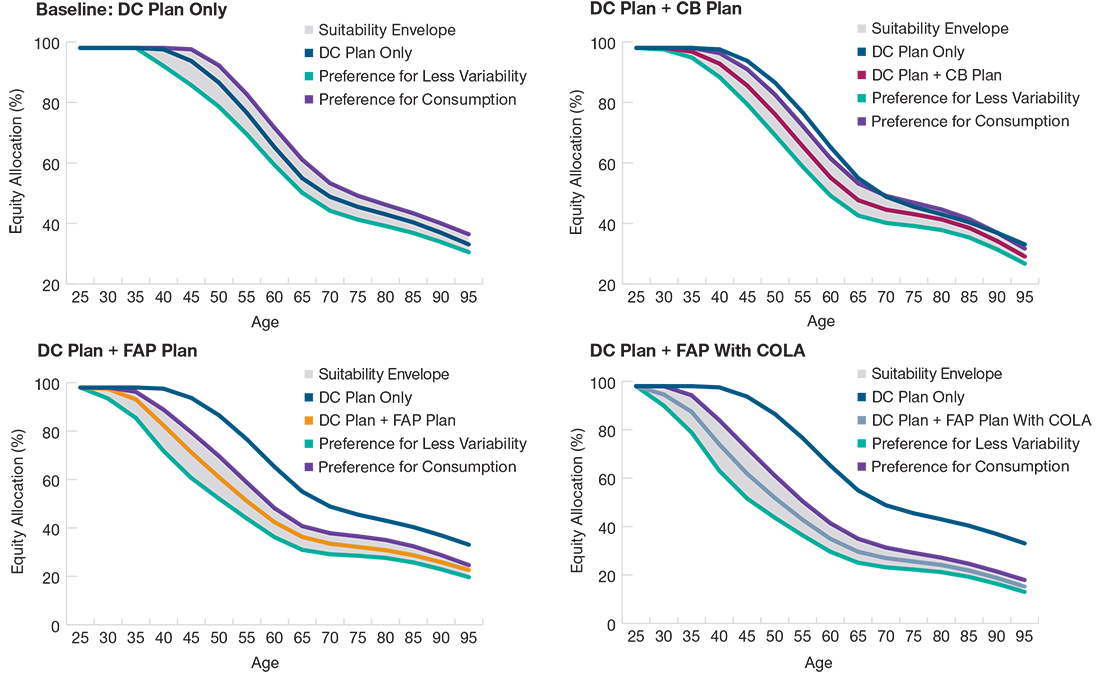
Rather than using one single set of assumed preferences, our practice is to vary them. This can produce a range of possible glide paths in our simulations that we call the suitability envelope. The boundaries of each of the envelopes shown in Figure 5 reflect slight adjustments to the specific parameter in our model representing the trade-off between consumption and wealth.
When we reran the simulations under different DB plan structures, we found that similarly sized suitability ranges were generated for all of them. This suggests that the initial results shown in Figures 1 and 2 were directionally robust, even for plan sponsors with different retirement objectives for their participants.
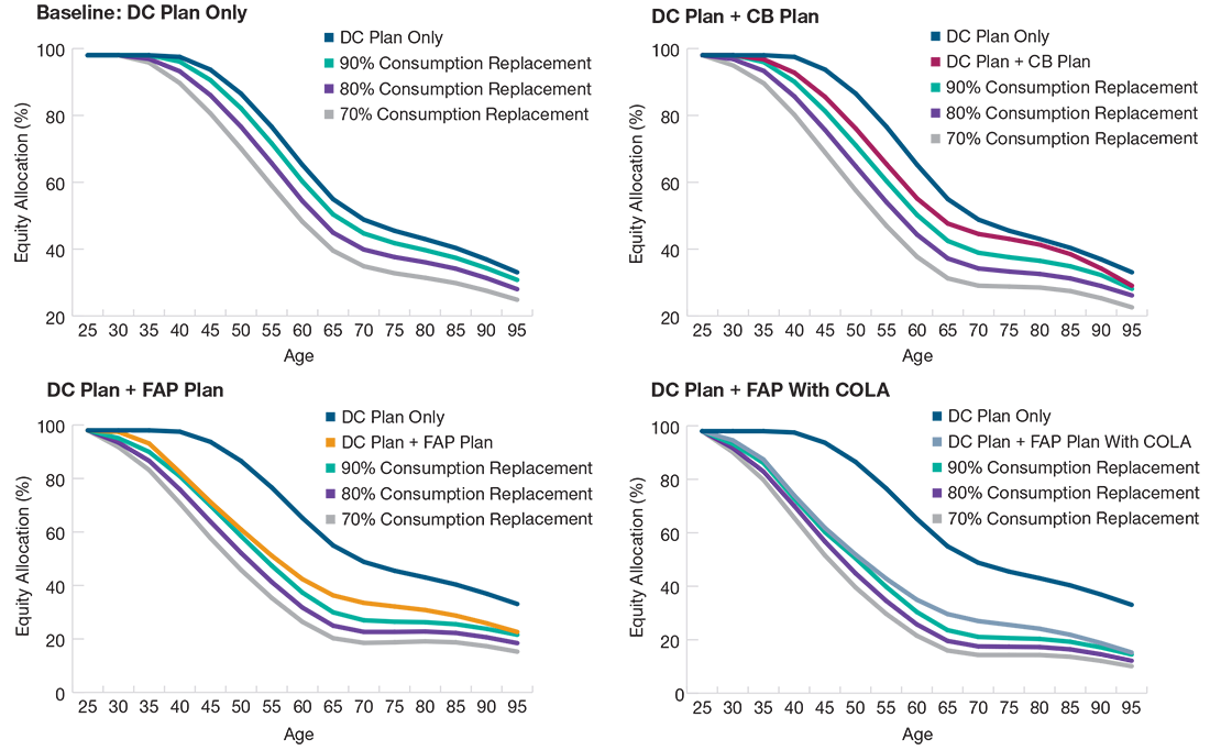
Another parameter we can adjust in our model is the percentage of preretirement consumption a participant is attempting to replace. The hypothetical glide paths shown so far in this paper incorporated our default assumption of a goal of fully replacing 100% of real preretirement spending. As we modified this target in 10% increments in our simulations, we again found that the model traced out comparable glide path ranges (Figure 6), confirming that the direction of the original analysis held even when different levels of retirement consumption were assumed.
Results Were Directionally Robust Regardless of Sponsor Preferences
(Fig. 5) Hypothetical suitability envelopes under differing wealth vs. consumption preferences
Results Also Were Robust Regardless of Income Replacement Objectives
(Fig. 6) Hypothetical suitability ranges under varying consumption replacement targets
Conclusions
DB plans come with a variety of features we have investigated here, most notably the form of the benefit payments. (Plan benefits also may include early retirement subsidies—a feature we intended to explore in a future installment of the Making the Benefit Connection series.)
Generally, the existence of an inflation-indexed benefit option, as is common in many U.S. public DB plans, will cause a glide path to de-risk the equity level more quickly during the accumulation phase compared with an FAP plan that only offers nominal benefits—a more common feature in corporate plans.
However, because cash balance beneficiaries often roll their lump-sum benefits into their DC plans at retirement but generally do not assume market risk on these assets until retirement, our model reduces equity exposure more slowly during the accumulation phase when there is a companion CB plan but reduces it more quickly during the later postretirement years as the full value of the CB lump-sum benefit is exposed to market fluctuations.
In our view, these nuances suggest that plan sponsors should carefully consider not only the retirement preparedness (wealth) generated by their DB plans, but also the pattern of accrual and the timing of the payouts provided. In our analysis, these results held regardless of plan sponsor preferences for wealth accumulation and consumption.
Appendix
Key Modeling Plan Design Parameters
Cash balance plan: The plan modeled throughout this analysis had the benefit structure shown in Figure A1, with the lump-sum benefit payable at retirement and rolled entirely into the companion DC plan.
The annual interest credit was assumed to be a minimum of 3% or the current yield on the U.S. 10-year Treasury note.
Hypothetical DC plan: Our starting assumption was a safe harbor plan design with the employer matching up to 100% of the first 3% of employee deferrals and 50% of the next 2%. We assumed all contributions were pretax and that contributions increased over time according to our proprietary deferral rate growth model.
Demographic analysis: We assumed that participant incomes grew in line with a proprietary salary growth model calibrated on the T. Rowe Price DC recordkeeping platform. Participants were assumed to retire at age 65 and begin withdrawing income to support a steady, inflation-adjusted level of spending over retirement.
DC objective preferences: DC plan sponsors have various investment focuses and desired planning horizons. These include the relative preference for consumption support versus balance variability modeled in Figure 5. Both levers are a part of our utility model and can be calibrated using intuitive and comprehensible metrics, such as weighted balance volatility.
Projections or other information generated regarding the likelihood of certain outcomes are not guarantees of future results. This analysis is based on assumptions, and there can be no assurance that the projected results will be achieved or sustained. Actual results will vary, and such results may be better or worse than the assumed scenarios.
(Fig. A1) Annual Pay Credit
| Age + Years of Service |
Pay Credit Percentage |
| Less than 40 |
4% |
| 40–50 |
5% |
| 50–60 |
6% |
| 60–70 |
7% |
| 70–80 |
8% |
| 80 or More |
9% |