The preceding paper in our Making the Benefit Connection series explored how suitable glide paths might differ between two otherwise identical DC plans when participants have varying levels of access to a sponsor’s DB plan.¹ In our simulations, we found that suitable glide paths for participants with access to both DB and DC plans typically had lower equity levels throughout the entire investment life cycle because of what we call the wealth effect—the reality that as retirees become better funded (wealthier), they have less need to expose themselves to riskier, more volatile assets in hopes of earning higher returns.

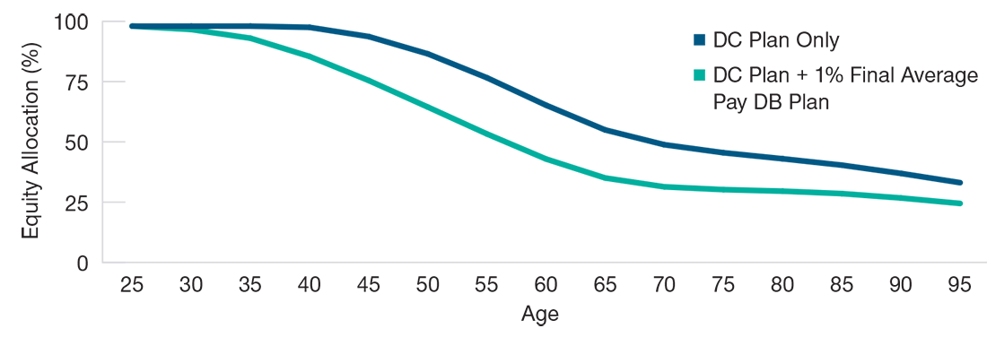
Compared with counterparts who only have access to a sponsor’s DC plan, participants who also have DB plan coverage should tend to be more amply funded for retirement, thanks to the value of their DB plan benefits. Figure 1 illustrates the potential impact of this wealth effect by comparing the optimal glide paths in our simulations for a hypothetical standalone DC plan and for the same DC plan when participants also were covered by a hypothetical companion DB plan.

The hypothetical DC plan shown in Figure 1 was assumed to be a safe harbor design featuring an employer match of up to 100% of the first 3% of salary in employee deferrals and 50% of the next 2%. The hypothetical companion DB plan offered a retirement benefit equal to 1% of the final five‑year average salary per year of service.²

In our simulations, we found that because participants with access to the hypothetical DB plan were better prepared financially for retirement, their DC target date glide path could maintain up to 23 percentage points less equity exposure and still give them a reasonably strong potential of meeting their retirement spending goals.

While the results in Figure 1 are interesting on their own, the hypothetical comparison used in our simulations admittedly was somewhat unrealistic. It assumed that the DB plan offering was strictly supplemental to the sponsor’s DC plan rather than a substitute for a more generous DC plan.

"Any sponsor will have a finite budget for retirement benefits, which raises numerous questions and implies potential trade‑offs."

However, plan sponsors designing retirement programs to serve as recruitment and retention tools ultimately are constrained in their design choices. Any sponsor will have a finite budget for retirement benefits, which raises numerous questions and implies potential trade‑offs.

• How can the benefit budget best be deployed to align with the organization’s retirement philosophy?
• Does the sponsor want to encourage employees to retire in their late 50s, their early/mid‑60s, or later?
• Should retirement benefits be tied to the success of the organization?
• How does the sponsor weigh the relative importance of retirement outcome predictability versus cost predictability?

Given these constraints, we believe that a realistic assessment of glide path suitability requires that a DB plan should not be evaluated simply as an additional benefit paired with an existing DC plan, but rather should be compared with an equivalent‑cost DC plan in isolation.

Identifying Equivalent‑Cost DB and DC Plans

Comparing benefit costs within a single plan type with the same structure can be relatively straightforward. For example, we can definitively say that a defined benefit plan that provides a retirement benefit equal to 1% of final five‑year average salary for each year of service is less generous than the same plan but with a 1.5% salary multiplier. Similarly, a DC plan with a 5%‑of‑salary non‑elective employer contribution is more expensive than a plan with a 3%‑of‑salary contribution.

However, cost equivalency becomes slightly more difficult to assess when comparing different designs within the same type of plan:

• A 1% final average pay plan, for example, is likely to cost more than a 1% career average pay plan because salaries for most employees will tend to increase throughout their working careers.
• Similarly, a DC plan that matches participant contributions dollar for dollar up to 6% of salary is likely to cost more than a DC plan that simply makes a non‑elective contribution equal to 2% of salary—although that might not be true if many employees don’t participate in the plan.

Determining cost equivalency across plan types (in this case, between DB and DC plans) adds another level of complexity to the exercise, requiring a myriad of assumptions—including, but not limited to, expected investment returns, interest rates, employee participation rates, deferral elections, salary growth rates, actuarial funding methods, participant mortality, estimated retirement ages, termination incidence, disability incidence, and more.

Additionally, funding mechanisms differ for U.S.‑based DB plans based on whether the plan is sponsored by a corporate or a government entity.³ These funding decisions are an additional wrinkle that needs to be considered in any cost comparisons.

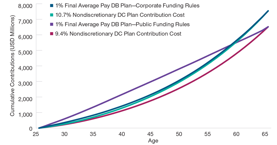
Different funding methods mean that sponsor contributions to a DB plan trust will be made at different points in the employment cycle, giving those investments differing amounts of time to generate the returns needed to pay future benefits.⁴ This nuance is subtle, but it is why there are multiple “equivalent cost” lines for the hypothetical DB plans shown in Figure 2, depending on how the plan sponsor was assumed to fund those benefits.

Based on insights gleaned from the aggregate behavior of the 2.2 million participants in T. Rowe Price’s recordkeeping database, our simulations indicated that the cumulative 40‑year cost of a hypothetical 1% final average pay DB plan (without service limit) based on corporate funding rules was approximately equal to the cost of a DC plan with a 10.7% salary match/non‑elective deferral. The 40‑year cost of an equivalent hypothetical DB plan based on public funding rules, meanwhile, was approximately equal to a DC plan with a 9.4% salary match/non‑elective deferral.

Glide Path Results

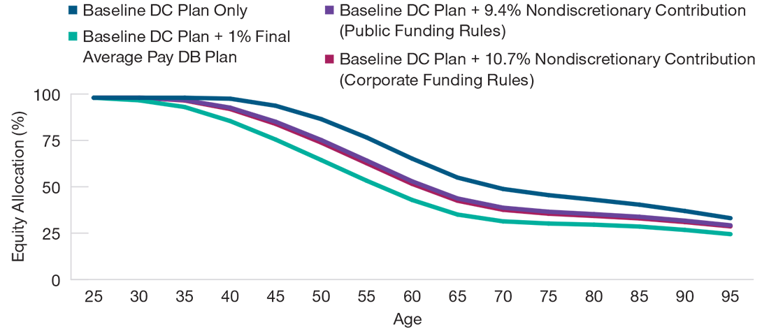
In our next set of simulations, we sought to control for potential differences in benefit richness (i.e., for the substitution effect⁵) by enhancing our baseline hypothetical DC plan. The enhanced plans offered the original matching formula but also included the additional nondiscretionary contributions (10.7% or 9.4%) required to equal the cost of our hypothetical DB plan under both corporate and public funding rules.

"...in our simulations, the wealth effect seemed to explain about half of the difference in glide path equity exposure caused by the existence of a DB plan."

In our simulations, these changes eliminated about half of the difference in optimal equity exposure between the baseline DC‑only glide path and the DC‑plus‑DB glide path (Figure 3).

Stated differently, the wealth effect seemed to explain about half of the difference in glide path equity exposure caused by the existence of a DB plan. In fact, a 20% nondiscretionary contribution was required in our simulations to generate a hypothetical DC‑only glide path with equity levels comparable to our combination of a baseline/safe harbor DC plan and the final average pay DB plan.

The other half of the difference in glide path equity was explained by the benefit accrual and payment structures themselves. A DC plan with nondiscretionary contributions provides extra savings during working years and then becomes the primary source of income for most participants after retirement (even though Social Security benefits typically replace a higher share of earnings for lower‑paid employees). A DB plan provides a relatively stable and secure source of retirement income that shields participants from market volatility. This should tend to reduce their reliance on their DC plans and other savings.

Under these circumstances, when the DC plan in our simulations provided benefits comparable in employer cost to the final average pay DB plan (in other words, fully reflecting the substitution effect), the optimal equity level in the DC‑only glide path still was higher than in a glide path designed for participants who also had access to the company’s DB plan.

By contrast, even when total benefit costs were comparable, providing part of that benefit in the form of a DB plan resulted in lower equity levels in the DC target date glide path in our simulations, particularly at the time of retirement. The DB plan benefit structure helped maintain wealth stability, which itself has potential utility value for participants.

Conclusions

In isolation, adding a hypothetical DB plan to an existing hypothetical DC plan substantially reduced the optimal equity allocation in the target date glide path in our simulations. However, looking at the DB plan in isolation overly simplified the trade‑offs that many plan sponsors actually face.

DB plan closures and freezes are continuing and not many new plans are being offered, particularly by larger employers. Instead, many plan sponsors are enhancing their DC plans, either by improving percent‑of‑salary matching rates or by increasing non‑elective contributions to offset the end of DB coverage.

"...DB plan coverage doesn’t necessarily make participants better funded relative to those who only have access to a DC plan, given that there is an implicit trade‑off at play."

To us, these trends indicate that DB plan coverage doesn’t necessarily make participants better funded relative to those who only have access to a DC plan, given that there is an implicit trade‑off at play. When we controlled for overall benefit costs in our simulations, we found that the impact of the DB plan on the optimal DC plan glide path still was to reduce equity exposure, but not by as much as if we had ignored the substitution effect entirely.

The substitution effect explains about half of the difference in glide path equity allocations in our simulations, with the remaining half a result of structural differences in benefit designs between the DB and DC plans that we analyzed. We think this finding could be useful for plan sponsors who want to look holistically at their retirement benefit structures and, more importantly, consider the impact of their DB plan on their DC plan glide path.

Appendix

Discussion of DB and DC Cost/Benefit Equivalence

Comparing benefit levels between DB and DC plans is a very nuanced analysis that requires significant actuarial assumptions. Even if these assumptions were fully realized and knowable (they are not), there are design elements embedded in different retirement plan structures that make apples‑to‑apples comparisons between two plan designs very challenging. While T. Rowe Price does not specialize in retirement plan design consulting, there are several broader thematic areas where we believe our insights into retirement income and glide path suitability might usefully be applied:

• asset allocation,
• behavioral alpha,
• lifetime income efficiency,
• benefit equivalency,
• expenses,
• risk of over‑ or underfunding.

Asset Allocation

An individual participant in a DC plan is investing for a fixed time horizon (their life expectancy), whereas sponsors of open DB plans can allocate investment risk with a going‑concern mindset. Target date strategies ordinarily de‑risk as participants get closer to retirement and then through retirement. DB plans potentially can maintain a higher risk budget for longer, possibly allowing the sponsor to “earn” more of the cost of the benefits they offer, rather than having to fund them through plan contributions. However, this potential relative advantage is not as large as it once might have been, given that many DC glide paths now start at higher equity allocations than is typically observed in public and corporate DB plan portfolios.

In addition, many corporate DB plan sponsors have chosen to de‑risk their allocations since the passage of the Pension Protection Act of 2006 to better align the marked‑to‑market volatility of their plans’ assets and liabilities. In our view, this liability‑driven investing approach is reasonable from a risk management standpoint but potentially limits market upside for these portfolios relative to ones with higher equity allocations.

Behavioral Alpha

DC plan participants—particularly those not invested in target date vehicles—may buy or sell risk assets at inopportune times. While some of these behavioral biases may also affect the decisions of DB plan investment committees, the governance structure of many DB plans potentially encourages more informed rebalancing and reallocation decisions, in our view.

Lifetime Income Efficiency

A DB plan sponsor pools mortality risk across participants and provides lifetime income from the plan. DC plan participants who want to annuitize their account balances, on the other hand, must solicit pricing quotes from insurance companies that offer annuities. These prices typically would include pricing provisions designed to discourage adverse selection and provide a profit for the insurance company.

The Internal Revenue Service (IRS) publishes the interest rates and mortality tables that qualified corporate DB plans use for actuarial equivalence. These assumptions may be more favorable for DB participants relative to DC participants who are seeking annuitization of their DC plan assets on their own. This difference in actuarial equivalence methodologies means that a dollar of retirement income potentially may be delivered more cost effectively by a DB plan sponsor compared with the annuity market.

Benefit Equivalency

Throughout our analysis, we have focused on comparing DB and DC plans of similar cost to the sponsor, based on the funding rules and methodologies prevalent among sponsors today. One alternative approach to assessing the substitution effect would be to compare plans that have similar benefit value equivalency instead of cost equivalency.

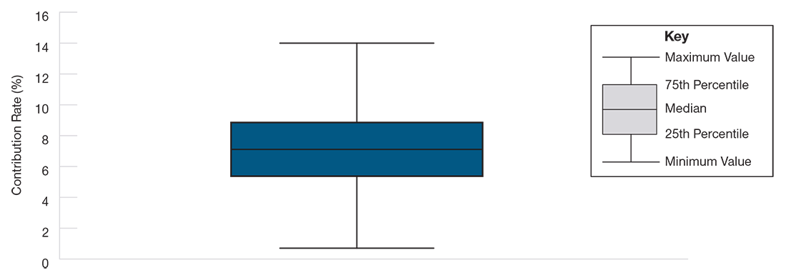
In our simulations, for example, a hypothetical DC plan with a nondiscretionary contribution rate equal to 7.4% of salary would, on average, provide the same present value of accrued benefits at retirement as the hypothetical 1% final five‑year average pay DB plan used throughout this paper. However, that figure is highly sensitive to the pattern and level of investment returns and interest rates. Figure A1 shows the range of equivalent nondiscretionary contributions required in our simulations to replicate the benefit value provided by the hypothetical final average pay DB plan.

Expenses

Collective trusts allow DC plan sponsors to enjoy some of the same economies of scale for investment fees that are available for the separately managed accounts more typically utilized by larger DB plans, potentially helping to keep DC costs reasonable for participants.

Both plan types have similar administrative expenses (legal, recordkeeping, regulatory filings, participant communications, etc.), although as premiums charged by the Pension Benefit Guaranty Corporation continue to rise for DB plans, DC plans may acquire a cost advantage in this area.

Similarly, actuarial costs are incurred by DB plan sponsors but not by their DC counterparts. However, the added administrative costs borne by DB plans typically are roughly offset by potentially higher DC plan investment fees, resulting in a wash from a cost/benefit perspective.

Over‑ or Underfunding

In our simulations, funding requirements for DB plans experienced much more year‑to‑year variability than those for DC plans. We believe this tendency helps explain the real‑world decline we’ve seen in sponsors offering DB plans.

Average investment returns—and, equally important, the volatility of those returns—are some of the most challenging assumptions to forecast, but also have material impact on cost‑equivalence estimation. Equity markets historically have been highly volatile, and in our simulations we have modeled funding policies that are consistent with both the IRS funding regulations for corporate DB plans and the annual contributions called for in Governmental Accounting Standards Board Statement No. 68 for public DB plans.

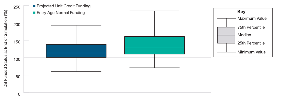
As shown in Figure A2, targeting a funding level of exactly 100% is quite challenging in the DB plan space, where underfunding during poor market years combined with the inability to recuperate past contributions during strong market years potentially creates a wide distribution of funded status outcomes at any forecast point.

In our simulations, a non‑negligible percentage of the outcomes resulted in overfunding of the hypothetical DB plan because we assumed that sponsors contributed additional funds during market drawdowns but didn’t have easy access to excess funds following periods of market strength.

DB plans also are potentially at risk for underfunding, particularly in the public plan space, where actuarially determined contribution amounts are not typically legislatively required. While this consideration does not necessarily impact glide path suitability or participant planning, it does make the “cost equivalence” comparison more difficult because, unlike DC plans, DB plans have some wiggle room surrounding contribution amounts and timing.

Key Modeling Plan Design Parameters

Hypothetical DB Plan: A final average pay plan that paid a single life annuity with the following benefit formula: normal retirement benefit at normal retirement date = 1% x the average of the final five years of pay x years of service.

For the purposes of this paper, we did not assume any subsidized early retirement benefits or cost of living adjustments. We plan to address these topics in future installments of the Making the Benefit Connection series.

Hypothetical DC Plans: Our starting assumption was a safe harbor plan design with the employer matching up to 100% of the first 3% of employee deferrals and 50% of the next 2%. We assumed all contributions were pretax and that contributions increased over time according to our proprietary deferral rate growth model. For our hypothetical public and corporate cost‑equivalent DC plans, we modeled nondiscetionary employer contributions of 9.4% and 10.7% of salary, respectively.

Key Assumptions About the Demographic Analysis: We assumed that participant income grew using a proprietary salary growth model calibrated on the T. Rowe Price recordkeeping platform. Participants were assumed to retire at age 65 and begin withdrawing income to support a steady, inflation‑adjusted level of spending over retirement.

The projections or other information generated regarding the likelihood of certain outcomes are not guarantees of future results. This analysis is based on assumptions, and there can be no assurance that the projected results will be achieved or sustained. Actual results will vary, and such results may be better or worse than the assumed scenarios.

Entry‑Age Normal Funding Method

More typically used by public pension plans, this funding method attempts to fund defined benefits as an equal portion of payroll across the participant’s expected future working lifetime. Any funding shortfall caused by investment underperformance relative to the discount rate is amortized over the remaining expected future working lifetime of the participant.

Projected Unit Credit Funding Method

Used for funding and accounting disclosures by most corporate pension plans, the projected unit credit funding method generally requires lower contributions earlier in a participant’s employment cycle compared with the entry‑age normal funding method. The current liability represents the ratio of current service to expected service multiplied by the present value of future expected benefits, reflecting discounting and decrementing. Any funding shortfall caused by investment underperformance relative to the discount rate is amortized over seven years to align with current IRS funding regulations.

Defined Benefit Assumptions

For the purposes of this paper, we assumed that the sponsor contributed the minimum of the normal cost plus an amortization of the underfunded balance, or zero if the plan was overfunded at the end of the prior year. We assumed a static asset allocation of 60% equity and 40% fixed income for this exercise, which produced an expected return slightly higher than the average 5% discount rate assumption used throughout our analysis. For this reason, the cost of the hypothetical DB plan was less than the present value of the benefits promised within the plan.